

Lessons from Fine Tuning a Convolutional Binary Classifier

Fine tuning has been shown to be very effective in certain types of neural net based tasks such as image classification. Depending upon the dataset used to train the original model, the fine-tuned model can achieve a higher degree of accuracy with comparatively less data. Therefore, we have chosen to fine tune ResNet50 pre-trained on the ImageNet dataset provided by Google.
We are going to explore ways to train a neural network to detect cars, and optimise the model to achieve high accuracy. In technical terms, we are going to train a binary classifier which performs well under real-world conditions.
Taken in a village Near Jaipur (Rajasthan, India) by Sanjay Kattimani http://sanjay-explores.blogspot.com
There are two possible approaches to train such a network:
- Train from scratch
- Fine-tune an existing network
To train from scratch, we need a lot of data — millions of positive and negative examples. The process doesn’t end at data acquisition. One has to spend a lot of time cleaning the data and making sure it contains enough examples of real world situations that the model is going to encounter practically. The feasibility of the task is directly determined by the background knowledge and time required to implement that.
Basic Setup
There are certain requisites that are going to be used throughout the exploration:
- Datasets
a.Standford Cars for car images
b. Caltech256 for non-car images - Base Network
ResNet — arXiv — fine-tuned on ImageNet - Framework and APIs
a. TensorFlow
b. TF Keras API - Hardware
a. Intel i7 6th gen
b. Nvidia GTX1080 with 8GB VRAM
c. System RAM 16GB DDR4
Experiment 1
To start with a simple approach, we take ResNet50 without the top layer and add a fully connected (dense) layer on top of it. The dense layer contains 32 neurons which are activated with sigmoid activator. This gives approximately 65,000 trainable parameters which are plenty for the task at hand.
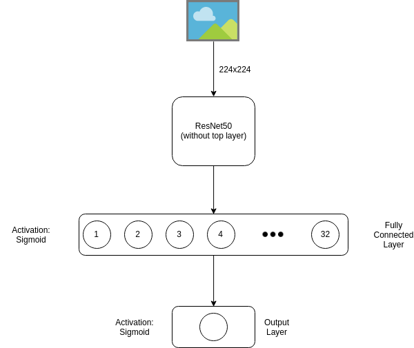
We then add the final output layer having a single neuron with sigmoid activation. This layer has a single neuron because we are performing binary classification. The neuron will output real values ranging from 0 to 1.
Data Preparation
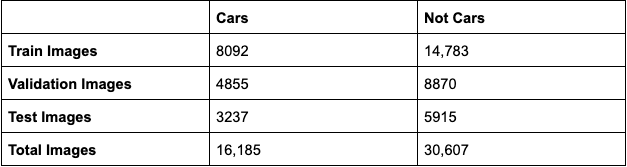
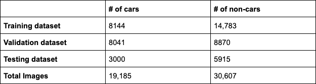
We are randomly sampling 50% of images as the training dataset, 30% as validation and 20% as test sets. Although there is a huge gap between the number of car and non-car images in the training set, it should not skew our process too much because the datasets are comparatively clean and reliable.
Hyper-parameters
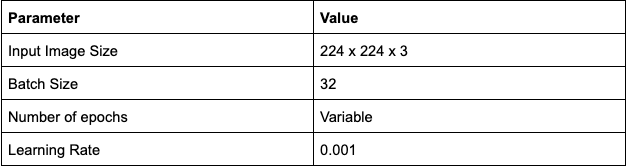
Results
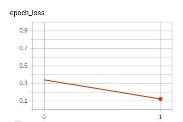
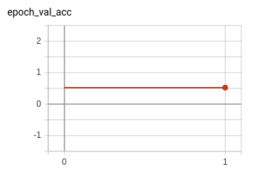
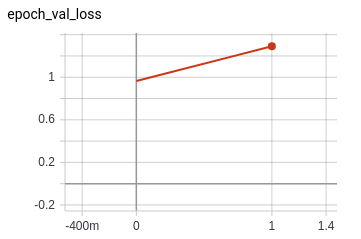
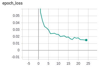
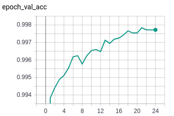
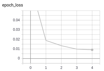
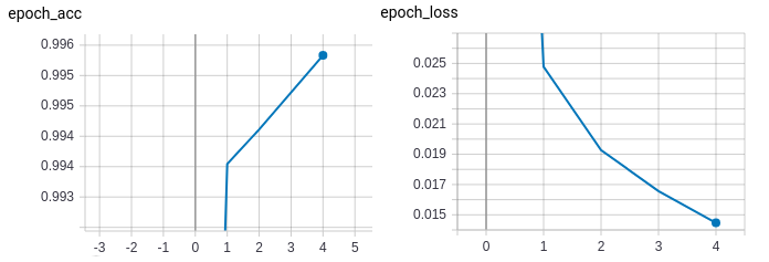
As a trial run, we trained for one epoch. The graphs below illustrate that the model starts at high accuracy, and reaches near-perfect performance within the first epoch. The loss goes down as well.

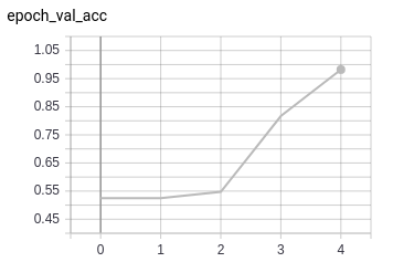
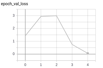
However, validation accuracy does not seem very good compared to the training round, and neither does validation loss.
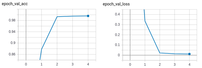
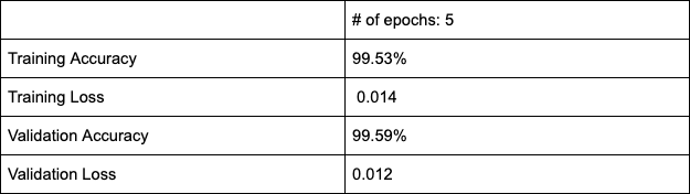
So, we ran for 4 epochs and were left with the following results:
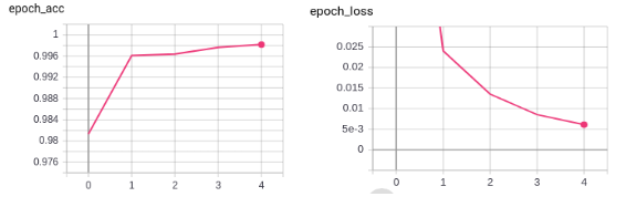
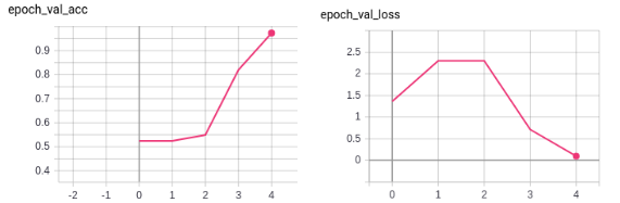
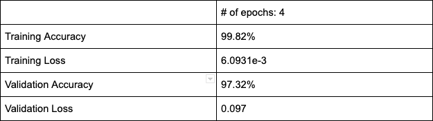
The model performs relatively well, except for the high degree of separation between training and validation losses.
Experiment 2
We decided to keep the model architecture the same as the one we used in the first experiment, using the same ResNet50 without the top layer and adding a fully connected (dense) layer on top of it containing 32 neurons activated with sigmoid activator.
Data Preparation
This is where the problem lay in the previous experiment. The train/validation/test data splits were random. The hypothesis was that the randomness has added more images of some cars, and too little of others, causing the model to be biased.
So, we took the splits as given by the Cars dataset and added 3000 more images by scraping the good old Web.
Hyper-parameters
Results
These results signify a substantial improvement in the validation accuracy when compared to the previous experiment.

Even though the accuracy matches fairly well, there is a big difference between the training loss and the validation loss.
This network seems more stable than the previous one. The only observable difference is that of new data splits.
Experiment 3
Here we add an extra dropout layer which provides a 30% chance that a neuron will be dropped out of the training pass. The dropout layer has been known to normalize models, to prevent possible biases caused by interdependence of neurons.

Since we have a comparatively huge pre-trained network and smaller trainable network, we could add more dense layers to see the effects. We did that and the model ended up achieving saturation in fewer epochs. No other improvements were observed.
Data Preparation
Just like in experiment 2, the default train/validation splits are taken.
Hyper-parameters
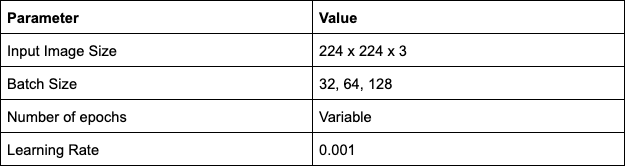
Here, we have run the model on a single learning rate but the value can be experimented with. We will talk about the effects of batch size on this network in the results section.
Results
The results here are with the batch size of 32. As seen, in 3 epochs the network seems to saturate (although it might be a bit premature to judge this).
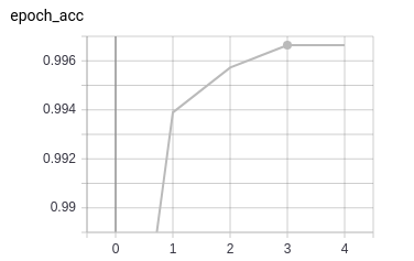
At the same time validation accuracy and loss also seem to be performing well.
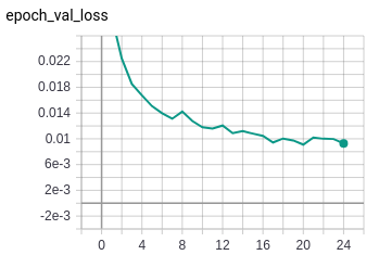
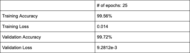
So, we increase the batch size to 128 hoping it would help the network find a better local minima and thereby giving a better overall performance. Here is what happened:
The model now performs reasonably well on both training and validation sets. The losses between training and validation runs are not too far apart either.
Model Drawbacks
Obviously, the model is not one hundred percent accurate. It does provide certain failed classifications as a result.
Conclusion
When we ran this model on the testing dataset, it failed on only 7 images out of car + non-car sets. This is a very high degree of performance accuracy and closer to production usage.
In conclusion, we can safely assert that dataset splits are crucial. Rigorous evaluations and experimentation with various hyper-parameters give us a better idea of the network. We should also think about modifying the original architecture based on the evidence provided by the various hyper-parameters.
Are you looking for a reliable technology partner for your ideas ? Talk to us